Binomial Distribution, the number of successes in n independent and identically distributed trials, rather than a specific value of the variable being observed.

For students who are confused by the concept of Binomial Distribution. At first, I was thinking that if X ∼ Binomial(10, 0.5), where n = 10 is the number of trials and p = 0.5 is the probability of success in each trial. What is the code x <- 0:10 and then dbinom(x,10,0.5) in the R means? Why the expection E(X) is not simply each value times its probability like we did previously?

The code x<-0:10 creates a vector of integers ranging from 0 to 10, inclusive. This vector represents the possible values of the number of successes, denoted by x, in a binomial distribution with parameters n=10 and p=0.5. The function dbinom(x,10,0.5) computes the probability mass function of the binomial distribution with parameters n=10 and p=0.5 at each value in the vector x. The output is a vector of probabilities, where each element represents the probability of observing the corresponding value of x in the binomial distribution.

For example, suppose we want to calculate the probability of getting exactly 5 heads in 10 coin tosses, where the coin is fair. We can use the binomial distribution with n=10 and p=0.5 to model this situation. First, we create a vector of possible values for the number of heads, from 0 to 10, using the x<-0:10 command. Then, we can use the dbinom() function to calculate the probability of getting exactly 5 heads, given the binomial distribution:

x <- 0:10

dbinom(5, 10, 0.5)

The output should be 0.2460938, which represents the probability of getting exactly 5 heads in 10 coin tosses, where the probability of getting heads is 0.5.

The most important concept which confused me here is that in the context of a binomial distribution, the value of x represents the number of successes in n independent and identically distributed trials, each with a probability of success p, rather than a specific value of the variable being observed.

Relative Frequency and Probability, What's The Difference?

 Relative frequency and probability are related concepts, but they are not exactly the same. Relative frequency refers to the proportion or fraction of times that an event occurs in a given set of data. It is calculated by dividing the frequency of the event by the total number of observations in the data set. For example, if we observe 50 heads in 100 coin tosses, the relative frequency of getting heads is 50/100 = 0.5 or 50%. Probability, on the other hand, refers to the likelihood or chance of an event occurring. It is a measure of how likely or unlikely an event is, and it is usually expressed as a number between 0 and 1 (or between 0% and 100%). Probability is calculated by dividing the number of favorable outcomes by the total number of possible outcomes. For example, the probability of getting heads on a fair coin is 0.5 or 50%.

The difference between relative frequency and probability is that relative frequency is based on observed data, while probability is based on a theoretical or assumed model of the underlying process. Probability is a mathematical concept that allows us to reason about the likelihood of events, even when we don't have access to the data or when the data is incomplete. Relative frequency, on the other hand, is a tool for analyzing the distribution of data and making inferences based on the observed patterns.

It is also incorrect for finding the expectation of a random variable from a relative frequency table. To find the expectation of a random variable, we need to multiply each value of the random variable by its corresponding probability and sum up the products. In a relative frequency table, the probabilities are given by the relative frequencies, which are obtained by dividing the frequency of each value by the total number of observations. Therefore, to find the expectation of a random variable from a relative frequency table, we need to first convert the table into a probability table by dividing the frequencies by the total number of observations.

The difference between x̄ (x-bar) and μ (mu)

 In statistics, the symbol x̄ (x-bar) represents the sample mean or average of a set of data. It is calculated by adding up all of the values in the sample and dividing by the total number of values in the sample. The Greek letter mu (μ) represents the population mean or average of a larger group of data that the sample is drawn from. It is calculated in the same way as x-bar, but it represents the true mean of the entire population, rather than just the sample.

The difference between x̄ (x-bar) and μ (mu) is that x-bar represents the average of a sample of data, while mu represents the true average of the entire population from which the sample is drawn. Because samples are inherently imperfect and may not perfectly reflect the larger population, x-bar and mu may be different from each other.

Reference
Yakir, B. (2011). Introduction to statistical thinking (with R, without Calculus). The Hebrew University of Jerusalem, Department of Statistics.

The Reasons Why Measurements May Not Be Perfectly Reproducible

About the reproducible of a sample, I reckon that there are several reasons why measurements may not be perfectly reproducible, even when the same phenomenon is being measured under apparently identical conditions:

i. Measurement errors

All measuring instruments have some degree of imprecision or error associated with them. For example, a ruler may not be exactly straight, or a thermometer may not be calibrated perfectly. These errors can accumulate over repeated measurements and contribute to variability in the outcomes.

ii. Environmental factors

Even seemingly small differences in the environment can affect measurements. For example, changes in temperature, humidity, or air pressure can influence the behavior of some measuring instruments.

iii. Human factors

The people conducting the measurements may introduce variability due to their own limitations. For example, they may have slightly different visual acuity or reaction times, or they may interpret the results differently.

iv. Inherent variability

Some phenomena are inherently variable, and measurements of them will naturally vary. For example, in biology, there may be natural variation in the characteristics of organisms, even within a single population.

v. Random chance: Finally, there is always an element of chance involved in any measurement. Even if all sources of variability were eliminated, there would still be some residual randomness that would make it impossible to achieve perfectly reproducible results.

Overall, it is important to recognize that variability in measurements is a natural and unavoidable aspect of scientific research. However, scientists use statistical methods to quantify and manage this variability, in order to draw reliable conclusions from their data.

Random Variables Are Used To Model Situations In Which The Outcome, Before The Fact, Is Uncertain

For this week’s discussion, let's consider an example of measuring the effectiveness of a marketing campaign using a random variable. The variable we might choose to measure could be the number of website visits generated by the campaign. The sample space for this variable would be the range of possible website visits, which could be any positive integer value. The probabilities associated with each value in the sample space would depend on the success of the marketing campaign. If the campaign is successful, we might expect higher probabilities for values near the upper end of the sample space, while a less effective campaign might have more uniform probabilities across the range of possible values.

Suppose the goal of the campaign is to generate website visits, and the marketing team has developed a plan to drive traffic to the website through a combination of social media advertising, email marketing, and search engine optimization. The team has set a target of 10,000 website visits over a one-month period for the campaign. However, due to the unpredictable nature of marketing, the actual number of website visits generated by the campaign may vary from this target.

To model this situation using a random variable, we could define the variable X as the number of website visits generated by the campaign over the one-month period. The sample space for X would be the set of all possible positive integer values that X could take on, from 0 to some upper limit. Let's say that we define the upper limit as 20,000 website visits. We can then assign probabilities to each value in the sample space based on our expectations for the success of the campaign. For instance, we might estimate that the probability of generating 10,000 website visits (our target) is 0.3, while the probabilities of generating fewer or more visits could be distributed according to a normal distribution with a mean of 10,000 and a standard deviation of 2,500. Using these probabilities, we can make statistical predictions about the likely range of website visits, and calculate the expected value and variance of the random variable X.

However, it's important to remember that any individual outcome is subject to random variation and unpredictable factors, even if the overall success of the campaign is well-modeled by the random variable X. For example, a major news event or a competitor's marketing campaign could impact consumer behavior in unexpected ways and result in more or fewer website visits than predicted. As a result, while random variables can be useful for modeling marketing effectiveness.

As mentioned above, a random variable is the future outcome of a measurement, before the measurement is taken. If someone claims to know the outcome of an individual observation of website visits generated by the marketing campaign, they are likely overestimating their ability to predict the outcome. While we can use the sample space and associated probabilities to make statistical predictions about the likely range of website visits, any individual outcome will still be subject to random variation. Factors outside of the campaign, such as seasonality, external events, or changes in consumer behavior, could impact the outcome in ways that are difficult to predict.

To summarize, random variables can be useful for modeling situations in which the outcome is uncertain due to random variation, such as marketing effectiveness. While the sample space and associated probabilities can help to provide insights into the range of possible outcomes, it is important to acknowledge that any single outcome is still unpredictable and subject to random variation.

Reference
Yakir, B. (2011). Introduction to statistical thinking (with R, without Calculus). The Hebrew University of Jerusalem, Department of Statistics.

Horizontal Stretches and Compressions of Functions

What happen if we consider changes to the inside of a function? As the figure blow shows that when we multiply a function’s input by a positive constant, we get a function whose graph is stretched or compressed horizontally in relation to the graph of the original function. If the constant is between 0 and 1, we get a horizontal stretch; if the constant is greater than 1, we get a horizontal compression of the function.

WHY ?  Let's take a closer look at the graph. Image that if inside the f(x), the x, is running 2 times faster or 2 times larger than the original x, the output f(x) will be 2x larger ?? The answer is NO. However, it will go 2 times faster to arrive the output that originally f(x) will reach. For example, for each output f(x), f(2x) only need 1/2 x to reach the output that f(x) does. In short, For each of the same output f(x), the inside change x, 2x, or 0.5x decide how fast the output f(x) will be reached.

Reference

Abramson, J. (2017). Algebra and trigonometry. OpenStax, TX: Rice University. Retrieved from https://openstax.org/details/books/algebra-and-trigonometry

Vertical Stretches and Compression of Functions

When we multiply a function by a positive constant, we get a function whose graph is stretched or compressed vertically in relation to the graph of the original function. But why?

That's because each of the same input have been changed to the output 2x or o.5 of the original functions.

Reference

Abramson, J. (2017). Algebra and trigonometry. OpenStax, TX: Rice University. Retrieved from https://openstax.org/details/books/algebra-and-trigonometry

Arc Length, Radius, Radians, and Trigonometric

 1.  Find the length of an arc in a circle of radius 10 centimeters subtended by the central angle of 50°

An arc length S is the length of the curve along the arc. Just as the full circumference of a circle always has a constant ratio to the radius, the arc length produced by any given angle also has a constant relation to the radius, regardless of the length of the radius. The radian measure is also depends only on the angle. A full revolution (360°) equals 2π radians. A half revolution (180°) is equivalent to π radians.

Convert the 50° to radians 

2.  Graph  on [-4π, 4π] and verbalize how the graph varies from the graphs of . 

A function that has the same general shape as a sine or cosine function is known as a sinusoidal function. One of the general forms of sinusoidal functions is y = Asin(Bx − C) + D, where A represents its Amplitude, B represents its Periods, C and D represents its shifts. In this case,  has only inconstant Amplitude X. Therefore, this function is expected to be a function that has the same period of   but with larger and larger Amplitudes. And, since the function  is repeating its values between the interval [-1, 1], when  or  , the function  will repeatedly has the value of X and -X. In fact, they are the intersections of these functions,  ,  , and 

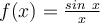
Graph   on the window [−5π, 5π] and describe freely what the graph shows.

Similar to the previous sinusoidal functions. One of the general forms of sinusoidal functions is y = Asin(Bx − C) + D, where A represents its Amplitude, B represents its Periods, C and D represents its shifts. This time, has only inconstant Amplitude . Therefore, this function is expected to be a function that has the same period of   but with smaller and smaller Amplitudes. And, since the function  is repeating its values between the interval [-1, 1], when  or  , the function  will repeatedly has the value of 1/X and -1/X. In fact, they are the intersections of these functions,  ,  , and

3. A 23-ft ladder leans against a building so that the angle between the ground and the ladder is 80°. How high does the ladder reach up the side of the building? 

If the ladder is lean against the TOP of the building and the building is vertically standing above the ground, we can use the sine function to solve this question. That is the heigh of the building is 

If the ladder is NOT lean against the TOP of the building and the building is vertically standing above the ground, then the height we just calculated is just a portion of the building and it represents where the ladder reach up the side of the building.

How can De Moivre's theorem be described? What is the scope of this theorem? Examples for roots and powers.

Finding powers of complex numbers is greatly simplified using De Moivre’s Theorem. 

According to the De Moivre’s Theorem 

If Z = r(cos θ + isin θ) is a complex number, then Zn = rn[cos(nθ) + isin(nθ)] 

where n is a positive integer. Zn = rn cis(nθ) 

How does it come from? To understand this theorem, we must know the products of complex numbers in polar form and the quotients of complex numbers in polar form first.

Recall that : 

    sin(α + β) = sin(α)cos(β) + cos(α)sin(β)

    sin(α – β) = sin(α)cos(β) – cos(α)sin(β)

    cos(α + β) = cos(α)cos(β) – sin(α)sin(β)

    cos(α – β) = cos(α)cos(β) + sin(α)sin(β)

 

 , 

 , 

,  

  = 

 ,